Sylvain's Blog

This blog post is a practical guide for analyzing AB test results easily and on the cheap. I want to emphasize on the word practical first. You will not find here in depth statistical explanations but more a practical view regarding methodologies you can use. On the cheap refers to the fact that I will be sharing with you tools, resources and code that you can use right now for free in Google Sheets and Apps Script.

You probably have to compute statistical significance all the time and buying a new AB test platform is not an option. It is either too expensive for your company or it will take time before you get the approval to invest in such a platform. So you have to do with what you have and if this sounds familiar, well welcome my friend! I have been there. I will share with you how you can dimension an experiment, calculate statistical significance, create a Bayesian AB test calculator just by leveraging Google Sheets.

As such this post is dedicated to Marketeers, UXers, Designers or any Data Driven person who wants to analyse the result of split tests without having to graduate from a PHD in Statistics first. Also, I believe this post can be invaluable to Data Analysts supporting Growth or Marketing departments. The Maths and Stats behind analysing split tests can sometimes also seem opaque to seasoned data practitioners.

I will be sharing my experience supporting various departments where AB testing is at the core of their inner way of working. I will go through the tools (built in Google Sheets for most of them but you will also find some Apps Script and Python) and techniques I use to answer the usual questions around dimensioning a test, analysing and reporting its results. In this post I will assume that you have a Data Engineering Team that can help you implement and track AB test data and all you need to do is analyse the results.

How to dimension an experiment when you do not have a tool?

When no experimentation platform is available to you, it is primordial to abide by a process in terms of designing experiments. With no tool on your side the easiest way is to rely on frequentist statistics fixed term horizon methodology. It is quite a mouthful but also very simple to use. I am going to share with you how you can leverage this methodology to define how long you should be running your test for.

In designing an experiment there are a bunch of metrics that you will have to surface. Most of the time it requires the help of a Data Analyst that might be able to grab the data for you. If you are data savvy and have access to your data warehouse, a bit of SQL will do.

To understand how long you should run an AB test for you need to:

define two statistical parameters, the statistical significance (alpha) and the power of the test (1 - beta). Usually alpha is set to 5% and the power to 80%. I would suggest that you stick to these numbers and do not over concern yourself with finding the “best” values for both,
understand the baseline conversion rate regarding the metric you want to improve: for example the number of website visitors clicking on a specific CTA. This is where your SQL skills or the help of a data analyst becomes handy,
define the Minimum Detectable Effect (MDE) for the test or in other words the minimum uplift you are expecting as a result of implementing the change. This is usually the metric where I see lots of stakeholders struggling with. “What is a good MDE?” is often a question I am being asked and in fairness there is a lot of guesswork that goes into defining it. However in the next chapter I will share some tips and techniques to help you make an informed decision.
Finally you also need to have an idea of the traffic coming into the page you are testing.

In summary:

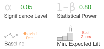
You can now calculate the sample size needed based on the abovementioned metrics and by comparing the sample size to your daily traffic you can then infer how many days you should be running the test for.

Here is a Google Sheets with the Power Analysis formula already set for you . Feel free to make a copy for your own use or even better create your own version.

Let’s use an example so you can familiarize yourself with the tool. Let’s say you are running an AB test on your landing page, and the goal is to make a CTA more visible to improve the click through rate.

You are going to have two variations: the control which is your landing page as is and the version of the landing page with the more visible CTA.
We select alpha at 5% and 1 - beta at 80%.
Just for the sake of the example we expect a relative increase of 10% in the conversion rate due to the implementation of the more “flashy” CTA. Once more, I will explain in the next chapter how you can define the MDE in an informed manner.
The baseline conversion rate regarding your CTA is around 12%.
Now imagine that your traffic on your landing is ~1000 visitors daily.

We input these numbers into our power analysis tool:

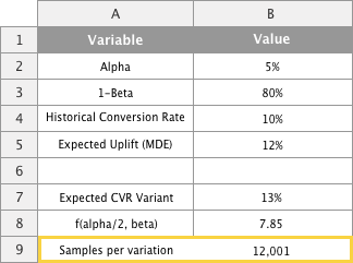
The tool tells us that we need around 12,000 visitors per variant, which is 24,000 in totals. We know that the traffic on our landing page is 1,000 visitors per day and as a consequence we know that we need to run the AB test for 24,000 / 1,000 = 24 days.

Pro Tip: usually the historical values that you use for power analysis might differ in reality when you run the test. It is always a good idea to add a few more days to make sure that you are compensating for unforeseen traffic variability. In the current case instead of running the test for 24 days I would probably run it for a full month. On top of “absorbing” the variability in traffic and making sure your test is not underpowered, gathering more traffic than previously scheduled can also allow you to detect smaller MDE than the one you were aiming at.

When and only when your test has run for the predefined amount of time that you should stop your AB test and gather the data. Using SQL directly or asking for the help of your favorite Data Analyst, you should then:

count the number of visitors for both the Control and the Variation(s) which will give you the sample sizes,
Count the number of visitors who converted (clicked the CTA) for both the Control and Variation(s),
Calculate the conversion rates by dividing 2 by 1.
Either compare the uplift (% difference between the variant and the control) against the MDE. If it is higher then you can conclude that the Variation is a winner. If it is lower then we do not have enough power to conclude that the Variation is a winner. Or you can also compute the p-value of the test and compare it against 5%. If the p-value is below 5% than the Variation is a winner.

How do you know what minimal detectable effect to select?

The reality is that you never really know what Minimum Detectable Effect (or MDE in short) to select in order to dimension your experiment. However there are a few things you can do in terms of getting close to a number that might be realistic or helpful.

If you have joined an existing Team which has already run tons of experiments, you can piggyback on the knowledge that has already been amassed. Accessing or creating a document summarizing every experiment that was run, with some descriptions of the page the test was run on, the measured effect (or difference between the Control and Variant) and whether it was statistically significant etc… can really help you assess the MDE of future experiments. Maybe you are about to run an AB test that was done before on a similar webpage: in this case you can use the effect found from that previous experiment as your best guess.

Now if you are joining a brand new Team and there is no existing knowledge that you can leverage to make educated guesses about your MDE, then there are probably two methodologies you can follow. The first one is basically to disregard all that experiment dimensionality calculation and run the experiment for two business cycles only. This can be a valid way to look at things if you work on “top of the funnel” initiatives like acquisition for example. In this case you are probably dealing with a lot of traffic so you can run every single of your AB tests for two weeks while still getting enough samples to detect very small effects.

The second solution and by far my preferred one is to follow a more data driven approach by leveraging what we learned from the previous chapter. It goes as follows:

Select different MDE: 2% relative increase, 5%, 10%, 20% …
Calculate the conversion rate for the variant based on the conversion rate for the control (baseline) multiplied by (1 + MDE), to make the impact clear.
For each MDE, and using the tool I have shared in the previous chapter, you can define what traffic would be needed for your experiment by dividing the total sample needed by the daily traffic.
Finally look at all the values and pick something that makes sense to you and your stakeholders.

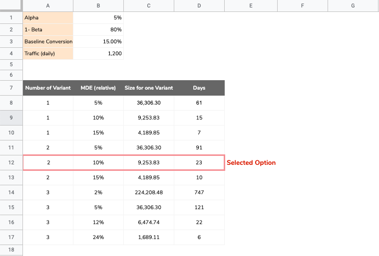
Select an appropriate Minimum Detectable Effect (MDE)

The boring and time consuming part here is having to compute the sample size for every single combination you are interested in. Like in the above example if you have a long list of different combinations (MDE, number of variations) you can spend a lot of time coming up with the sample size and test duration figures.

In this blog post I share some Apps Script code to automate all the calculations for you. Neat right? Now all you need to do follow the steps in the post and you are all set!

How to calculate statistical significance when you do not have a tool

Calculating statistical significance is not complicated and does not necessitate an advanced solution. It can be done from Google Sheets quite simply. If we take the example of comparing two conversion rates (control vs variant) here is a template that you can use. If the difference is statistically significant (based on your choosen alpha) then the Google Sheets will tell you so on cell B14.

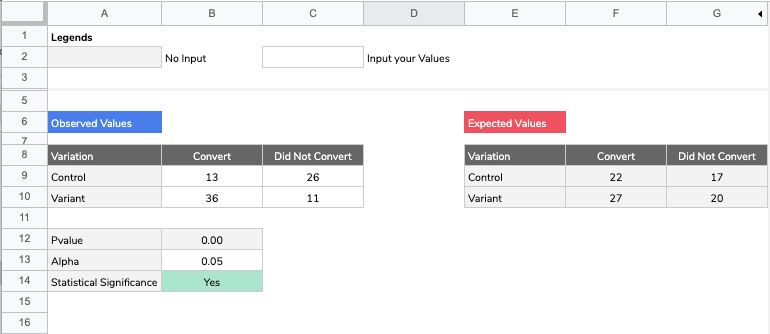
Statistical significance calculation for conversion rates

Let’s see what’s under the hood. First of all we are using the Chi Square Test (a mouthful I know). It is basically a test that will compare the data you have gathered against what your data would have looked like if the variant was similar to the control (in other words in the case where there is no effect at all due to the change you have implemented).

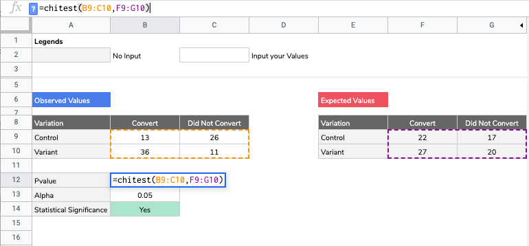
To work the Chi Square test needs you to transform your original dataset to compute the figures for the case where there is no effect whatsoever - which I called the Expected Values in the Google Sheets. The process would look something like:

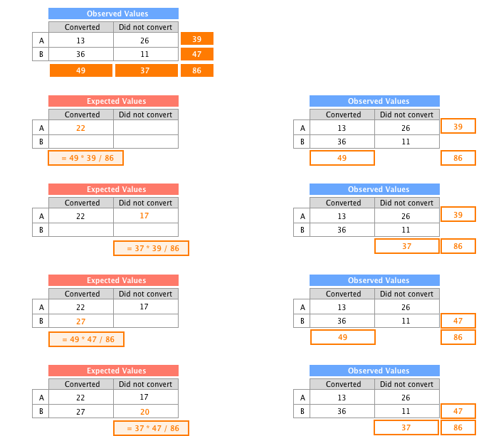
Once you calculated your p-value you can directly compare it against the significance level alpha (do not overthink it and pick 0.05, but whatever you choose make sure it is the same value as the alpha you selected for dimensioning your experiment). If your p-value is less than alpha then you can conclude that the variant is better than the control.

The next natural question is by how much is it better, and we do need to be careful on how we report it. This is what we are going to tackle in a couple of chapters from here.

For the moment, if your want to know in details how to calculate statistical significance not only for conversion rates but also for continuous variables, using either Google Sheets or Python, here is below a list of ressources:

In the next chapter I am going to go through analysing the result of an AB test and move beyond the black and white interpretation that is often required when we work in a professional setting as opposed to an academic one.

Interpreting the result of an AB test - Deep dive

All the methodologies and templates we have been through so far are all related to the frequentist world. Whithin such a setting, an AB test has implicitly two hypothesis:

The null hypothesis, which is the “contrarian” view for a test: we assume that the variant has no effect whatsoever on the metric we are interested in and is not better than the control.
The alternative hypothesis, the case we want to prove. This is the hypothesis where we assume that the variant has indeed an effect and improve the metric we are interested in.

When we calculate the p-value we are within the premise of the null hypothesis. We assume that the change implemented has no effect, and in this context we can interpret the p-value as a measure of “surprise”. It tells us how surprising the result is - in other words how surprising the difference between the variant and the control is - in a world where we assume that there should be no effect at all.

If the p-value is less than the significance level alpha we say that the result is so surprising that we have enough evidence to reject the null hypothesis and accept the alternative hypothesis. It does not necessarily mean that the alternative is true for sure. There still is a 5% chance (the significance level alpha) that we are facing a false positive: a case where we conclude that the Alternative Hypothesis is true when actually it is not.

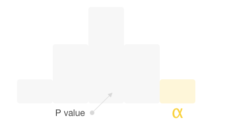
If the p-value is more than the significance level alpha then we say that we do not have enough evidence to reject the null hypothesis. We can not confirm that there is an effect, nor can we say that the null hypothesis is true, we just can not conclude anything unfortunately. In such a case, one should not reject the logic behind implementing the test in the first place and take the rejection as an indication that the change tested was not bold enough and needs to be reviewed, improved or tweaked.

How to report the difference between the Control and the Variant?

With frequentist statistics, we can only answer one question and one question only through an AB test: is the variant better than the control? Yes or No and that is it.

I have seen countless Data Analysts (I should include myself) and Product Managers making the same mistake which is to use the AB test result to estimate what the real uplift is or what the real difference in conversion rates between the two variations is.

The reality is that the uplift or the difference calculated from the test is likely to be over optimistic. Think about what would happen if you were to run the same AB test a hundred times. You would find some tests that failed to reach statistical significance, as well as a wide variety of numbers reported for the uplift from one test to another.

The goal is to set expectations right in our stakeholders’s mind and from my experience being cautious here is the right approach. There two ways to report on an AB test performance:

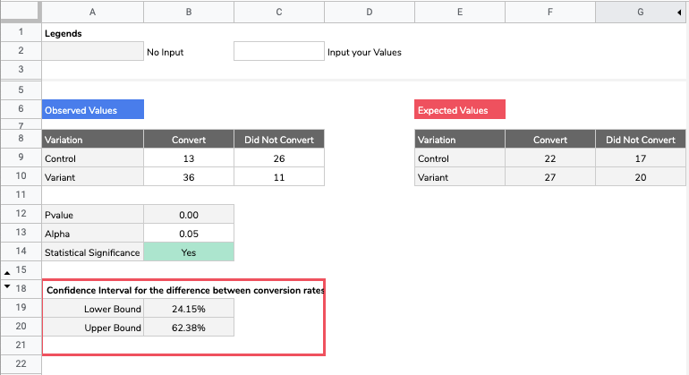
Report a confidence interval. A confidence interval tells you that if we were to run the same AB test a 100 times, the real difference between the Control and the Variant would be found within that interval 95 times. Usually this metric is often misunderstood and not well received by decision makers as it gives an interval of values without stating which value in the interval is the most likely. Here is a way you can compute the confidence interval for conversion rates, and the explanations of the formula used can be found here.

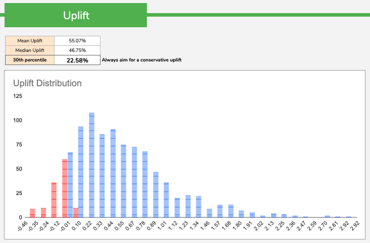
Analyse your ABtest using Bayesian Statistics

My favorite way of reporting an uplift is by using Bayesian Statistics. Bayesian Statistics help you define a probability distribution for the uplift. Since you have a probability distribution you can easily summarise that distribution by using the mean, the median or a percentile. My favorite one would probably be the 30th percentile as more conservative than the mean or median (remember we want to be cautious here and set lower expectations for our stakeholders). This method has the advantage of providing one value as opposed to an interval like in the previous case.

How to deal with small sample sizes?

The frequentist approach unfortunately does not work well when we deal with small samples. More often than not, when computing how long an experiment should run for one might find out that due to the low amount of traffic coming to the page the test would have to run for an unrealistic amount of time.

In such a case the frequentist approach here does not offer any insights. Either we run the test for the required period of time and then check the p-value but as discussed this is no longer an option due to the low traffic. Or we decide to run the AB test for two business cycles and compute the p-value afterwards. In that latter case it is very likely that the p-value is going to be meaningless (automatically more than 5%) - unless a “once-in-a-lifetime” effect is detected.

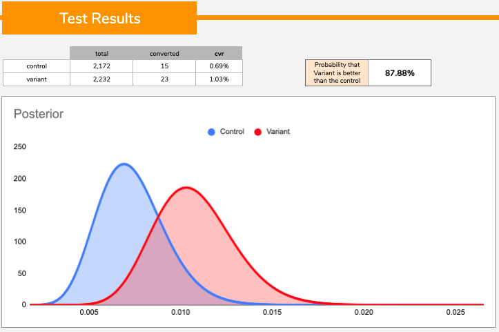
In such a scenario I find the Bayesian approach to be most helpful . It provides a probability that the variant is better than the control, no matter how small the sample size. You can then define a level of risk you are willing to accept. For example if the probability that the variant beats the control is higher than, say 90%, then conclude that the variant is a “winner”.

I do not advocate for a specific cut off point here, it is for anyone to make up their minds on the level of risk they are ready to accept. However, due to the small sample size it is also very likely that the result reported by Bayesian statistics stays quite low and rarely reaches a high probability level (above the 90% threshold for example), unless the effect of the change is very impactful. Small sample size equates to high variability. Now because Bayesian statistics provides a number we still have “something” we can use to make an informed decision based on the level of risk we are happy to take.

Pro Tip: regardless of the statistical methodology we use it is important to remind ourselves that, when dealing with small sample sizes, we need to make sure we maximize our chances to capture the "signal" by:

focusing on bold / impactful changes,
focusing on aeras / pages with the most traffic,
avoiding multi variant testings and sticking to one variant only, not to dilute the traffic,
lowering the statistical threshold (either statistical significance alpha in the frequentist setting, or our risk level when it comes to Bayesian statistics).

Summing it all up

If you do not have access to a modern experimentation platform but have the help of data engineers to technically set an experimentation up and track the data, measuring the result of an AB test can easily be done, on a cheap, leveraging Google Sheets, Apps Script or Python.

In a nutshell, the high level steps should be to:

always dimension your experiment to understand how long it should be running for.

Determine the appropriate MDE
Compute the sample size

Once the sample size needed is reached: stop the test and analyse the results.
Report whether the variant is better than the control. If that is the case beware of over-optimism when sharing uplifts or differences in conversion rates. Use either:

confidence intervals
or Bayesian statistics to report on a simple point estimate.

If dealing with small sample sizes, Bayesian statistics is more helpful than Frequentist statistics and provides an output than can be interpreted.