About the Central Limit Theorem

What is the Central Limit Theorem?

If we consider a random sample of n observations taken from any population with a given mean and standard deviation, if n is big enough (usually larger than 30), then the sampling distribution of the mean is approximately normal, centered on the population mean. This is what the Central Limit Theorem (or CLT) states.

Differently put, let’s say we make several “copies” of a random variable with any probability distribution. If the number of copies is big enough, then the average of them all will have a probability distribution that approximately follows a bell curve.

Implications of the Central Limit Theorem

Usually we take a sample from a population because we want to assess a characteristic of that population, like the mean concentration of a specific chemical in drinking water for example. Our sample serves as a way to estimate that characteristic. It is to be noted that the larger the sample size, the more precise our estimate is. In other words the larger the sample, the closer the sample mean gets to the population mean: it becomes a better estimate.

Intuitively this makes sense, as the average of many measurements of the same characteristic that we want to determine, is more accurate than a single measurement for example. The random errors inherent to the measurements tend to cancel each other out.

The central limit theorem also has another very important application in hypothesis testing as the normality assumption will tell us which statistical test to use. If we have a sample big enough, then we can assume normality and use a z-test; while if the sample is small then we would use a t-test instead.

Often sample sizes bigger than 30 suffice to assume that the Central Limit Theorem kicks in, but in fact, the more skewed the population distribution is, the larger the sample needed must be to satisfy normality.

Demonstration of the Central Limit Theorem

Let's load some packages first.

import pandas as pd
import numpy as np
import matplotlib.pyplot as plt
import statistics
import random
import seaborn as sns

Then we simulate a very skewed population distribution using the exponential:

sns.set(style="white", palette="muted", color_codes=True)

distributions = []
sum_random_var = 0
xbar = 0

sample_size = [1, 5, 15, 30, 200, 1000]
fig, ax = plt.subplots(3,2, figsize = (10, 7))
row, col = 0, 0

for s in sample_size:

    for n in np.arange(s):
        # Exponential distribution
        distributions.append(np.random.exponential(2, 10000))
        sum_random_var += distributions[n]

    xbar = sum_random_var / s

    sns.distplot(xbar,
                 label = 'n = ' + str(s),
                 ax = ax[row][col])

    sns.distplot(np.random.normal(np.mean(xbar), statistics.stdev(xbar), 1000000),
         hist = False,
         color = 'r',
         label = 'Normal',
         kde_kws={'linestyle':'--'},
         ax = ax[row][col])

    if col == 1:
        col = 0
        row += 1
    else:
        col += 1

ax[0][0].set_title("Exponential Random variable")
plt.show()

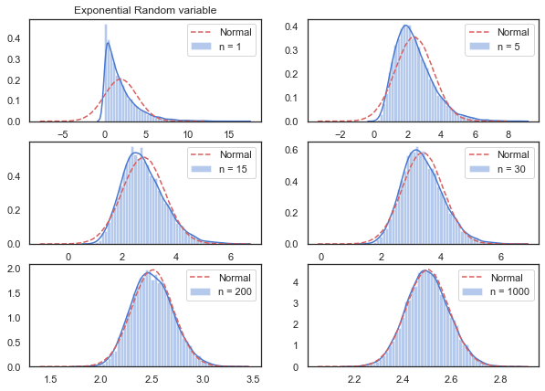
With a sample size of 15 we are quite close to the ideal bell curve represented in dashed red lines. However it does take a lot more samples, maybe somewhere between 30 and 200 to obtain a probability distribution that is more symmetrical and Gaussian.

Now let’s look at a binomial probability distribution that can simulate a toss coin or a conversion rate (traffic landing on a web page and clicking (or not) on a CTA for example).

distributions = []
sum_random_var = 0
xbar = 0

sample_size = [1, 5, 15, 30, 200, 1000]
fig, ax = plt.subplots(3,2, figsize = (10, 7))
row, col = 0, 0

for s in sample_size:

    for n in np.arange(s):
        # Binomial distribution
        distributions.append(np.random.binomial(1, 0.5, 1000))
        sum_random_var += distributions[n]

    xbar = sum_random_var / s

    sns.distplot(xbar,
                 label = 'n = ' + str(s),
                 ax = ax[row][col])

    sns.distplot(np.random.normal(np.mean(xbar), statistics.stdev(xbar), 1000000),
         hist = False,
         color = 'r',
         label = 'Normal',
         kde_kws={'linestyle':'--'},
         ax = ax[row][col])

    if col == 1:
        col = 0
        row += 1
    else:
        col += 1

ax[0][0].set_title("Binomial Random variable")
plt.show()

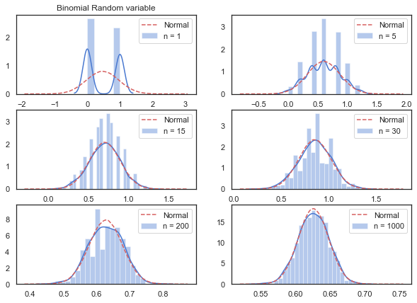
With 15 samples we are very close to the shape of a normal distribution which is quite astonishing.

It always amazes me that in practice the sample size does not need to be big for the CLT to be verified. A sample of size 30 suffices in most cases even when dealing with very skewed datasets. However the larger the sample size, the better: it ensures a tighter confidence interval and as such a more precise estimation of where the true parameter we are estimating lies.